Basics

In this notebook, we introduce basic ways to read, show, explore and save images.

%matplotlib notebook
from PIL import Image
import numpy as np
import matplotlib.pyplot as plt
from matplotlib import cm
from scipy import ndimage
from IPython.display import YouTubeVideo
import os

Preamble

Before going into the technical details, we strongly recommend these two videos from the excellent YouTube channel Dirty Biology:

Loading an image

To read an image with Python, the easiest way is to use the Python Image Library (PIL) which provides the basic tools.

Required files

Before using this notebook, download the image rabbit.jpg

The following code will work if the image is located in the same directory as the notebook itself. First, let’s check if the file rabbit.jpg is in the current directory.

files = os.listdir("./")
if "rabbit.jpg" in files:
    print("Ok, the file is in {0}".format(files))
else:
    print("The file is not in {0} , retry !".format(files))

Ok, the file is in ['.ipynb_checkpoints', 'image_processing_basics.ipynb', 'blobs.jpg', 'blob_orientation.ipynb', 'rabbit.jpg', 'support_material.md']

Now let’s read it using Python Image Library (aka PIL):

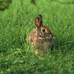
im = Image.open("rabbit.jpg")
im

Numerical images

There are mainly two kinds of numerical images:

• Vector images composed of basic geometric figures such as lines and polygons. They are very efficient to store schemes or curves. They are generally stored as .svg, .pdf or .eps files. In this tutorial, we will not work on such images.

• Raster images, also called bitmaps in which data is structures as matrix of pixels. Each pixel can contain from 1 to 4 values called channels. Images can then be sub classed by their number of channels:

  • A single channel image is called grayscale,

  • Most color images use 3 channels, one for red (R), one for green (G) and one for blue (B). They are called RGB images.

  • Some image formats use a fourth channel called alpha corresponding to the transparency level of a given pixel.

In the following, we focus on raster images. In the current image, the channel structure can be obtained as follows:

From image to numpy

In practice, we will manipulate the images in the form of arrays. With Python, the numpy library is the essential tool for this task. It is therefore necessary to know how to switch easily from an image to arrays and vice versa.

Now, the channel data can be extracted as follows:

R, G, B = im.split()  # Three channels: Red, Green and Blue
R = np.array(R)
G = np.array(G)
B = np.array(B)

fig, axes = plt.subplots(nrows=1, ncols=3)
axes[0].set_title("R")
axes[0].imshow(R, "gray")
axes[0].axis("off")
axes[1].set_title("G")
axes[1].imshow(G, "gray")
axes[1].axis("off")
axes[2].set_title("B")
axes[2].imshow(B, "gray")
axes[2].axis("off")
plt.show()

At this stage, an image is no more than a matrix generally made up of unsigned 8-bit integers (np.uint8). A color image is therefore made up of 3 grayscale images corresponding to the 3 channels:

R

array([[ 79,  86,  97, ...,  79,  70,  64],
       [ 72,  76,  84, ...,  97,  93,  87],
       [ 69,  71,  75, ..., 107, 101,  94],
       ...,
       [120, 115, 101, ...,  73,  64,  38],
       [130, 109,  81, ...,  73,  58,  31],
       [113,  84,  60, ...,  72,  68,  53]], dtype=uint8)

From numpy to image

Let’s see now how to switch back from an array to a real image.

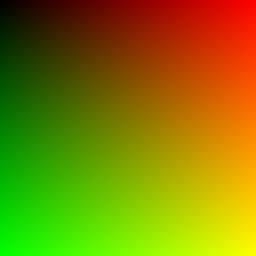
r2 = np.arange(256).astype(np.uint8)
g2 = np.arange(256).astype(np.uint8)
R2, G2 = np.meshgrid(r2, g2)
B2 = np.zeros_like(R2).astype(np.uint8)

im2 = Image.fromarray(np.dstack([R2, G2, B2]))
im2

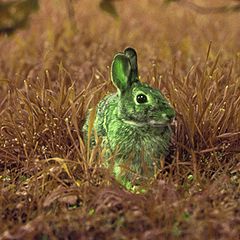
Let’s apply that to the rabbit image. For example, we can switch channels:

im3 = Image.fromarray(np.dstack([G, R, B]))
im3

How a filter is applied to an image ?

This video from the excellent YouTube channel 3Blue1Brown explains how a filter is applied to an image through a convolution operation. An example with the application of a Gaussian filter is presented.