Conway’s Game of Life#

Part 1: Introduction#
What’s the game of life?#
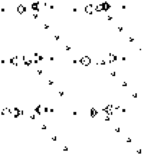
The game of life (GoL)is not a game per se. It is one of the first cellular automata. It can be visualized as a chessboard of arbitrary size in which each cell can exist in two states (dead=0 or alive=1). The game has an evolution rule that makes the state of its cell change with each time step. This rule is purely deterministic (which implies that there is no randomness in this game) and is based on the number of living Moore neighbors of each square.
This rule can be written as follows:
Birth (B): if a dead cell has 3 neighbors, it becomes alive 1. It remains dead 0 otherwise.
Survival (S): If a living cell has 2 or 3 neighbors of Moore, it survives thus remains 1, it dies and becomes 0 otherwise.
The rule of the game of life can be generalized as B3/S23. You can visualize the game graphically on the following simulator: https://bitstorm.org/gameoflife/
Further readings#
Part 2: Counting living Moore neighbors#
Our goal is to animate the game of life at a sufficient speed. Typically, a 200x200 grid should be able to be run in real time, i.e. 25 frames per second. The speed of your code execution must therefore be sufficient. Try counting Moore’s living neighbors on a small grid at first before moving to a larger one.
We can easily create a random binary matrix usin numpy
cells = np.random.randint(2, size=(5, 5))
cells
array([[1, 0, 0, 0, 0],
       [0, 0, 0, 1, 0],
       [1, 1, 1, 0, 0],
       [1, 1, 0, 1, 1],
       [0, 0, 0, 0, 1]])
plt.figure()
plt.imshow(cells, cmap=cm.gray)
plt.colorbar()
plt.show()
Now, you need to find a way to calculate the number of living (1) neighbors around every cell.
Tips:
Try several methods and determine which one is the best for you,
The use numpy’s slicing and striding methods can help,
Alternatively, numba can be an interesting solution in terms of performance, see 5 min to Numba.
Boundary conditions are importants.
Neighbors counts can be stored in a matrix like the following one:
neighbors = np.zeros_like(cells)
neighbors
array([[0, 0, 0, 0, 0],
       [0, 0, 0, 0, 0],
       [0, 0, 0, 0, 0],
       [0, 0, 0, 0, 0],
       [0, 0, 0, 0, 0]])
## Part 2: Creating a class
In what follows, we propose to model the game of life by a class of which the method of calculation of the neighbors that you have just written would be a method. Here is a basic code snippet that you can use as inspiration to move forward.
class GoL:
    """
    A game of life class.
    """

    def __init__(self, cells):
        self.cells = np.array(cells)

    def __repr__(self):
        return "<GoL with {0} cells>".format(self.cells.size)

    def count_living_neighbors(self):
        """
        Counts the number of living neighbors of each cell.
        """
        # to be completed.
        return

    def evolve(self):
        """
        make an evolution step forward.
        """
        # to be completed.
        return


g = GoL(cells)
g
<GoL with 25 cells>
Part 3: Animate your Game of Life !#
In the following example, we provide you with a class which is not related to the game of life but which consists of similar methods. It shows how to make an animation. Use it as an inspiration to animate your game of life.
class AliasingImage:
    """
    Creates a aliasing illusion.
    """

    def __init__(self, size=(5, 5), depth=8):
        self.size = size
        self.depth = depth
        lx, ly = size
        x = np.arange(lx)
        y = np.arange(ly)
        self.f = 1.0
        self.df = 0.07
        self.X, self.Y = np.meshgrid(x, y)
        self.evolve()

    def evolve(self):
        """
        Randomizes the image
        """
        f = self.f
        self.image = np.cos(2 * f * self.X) * np.sin(2 * f * self.Y)
        self.f += self.df


ri = AliasingImage(size=(50, 50))


def updatefig(*args):
    ri.evolve()
    im.set_array(ri.image)
    return (im,)


fig, ax = plt.subplots()
ax.axis("off")
im = plt.imshow(ri.image, interpolation="nearest", cmap=cm.gray, animated=True)
anim = animation.FuncAnimation(fig, updatefig, frames=40, interval=50, blit=True)
# plt.show()
plt.close()
anim
Part 4: Other rules#
The game of life can be generalized and other rules give surprising and interesting results from a mathematical point of view. Some of them include simple structures capable of cloning themselves, which reminds us of DNA in chemistry.
Modify your work in order to be able to simulate other rules easily.


