Practical Work: Steel microstructure

In this tutorial, you will study the microstructure of an HSLA steel.

Required files

Download the image file HSLA_340.jpg and put it in the same folder as this notebook.

Introduction

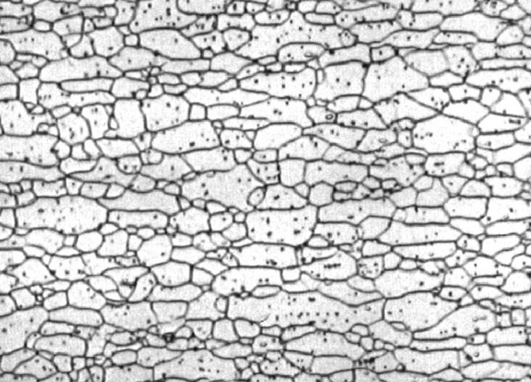
This image is a micrograph of a high-strength low-alloy (HSLA) steel. The image was taken using a scanning electron microscope (SEM) and shows the microstructure of the steel. The microstructure shows grains and separated by grain boundaries. The grains are regions of the material where the atoms are arranged in a regular pattern. The grain boundaries are the interfaces between the grains. The size of the grains and the distribution of the grain boundaries are important for the mechanical properties of the material. For example, the Hall-Petch equation relates the yield strength of a material to the average grain size.

Ressources

• Orientation and aspect-ratio with Positron

• Region properties with Scikit-Image

Objectives

In this tutorial, we will measure the grain size as well as the grain shape factor and the grain orientation.

Tasks

# IF USING JUPYTER LAB, USE THE FOLLOWING COMMAND:
%matplotlib widget
# IF USING JUPYTER NOTEBOOK, USE THE FOLLOWING COMMAND:
# %matplotlib notebook

from PIL import Image
import numpy as np
import matplotlib.pyplot as plt
from matplotlib import cm
from scipy import ndimage
import pandas as pd
import os

name = "HSLA_340.jpg"
workdir = "./"
files = os.listdir(workdir)
if name in files:
    print("Ok, the file is in {0}".format(files))
else:
    print("The file is not in {0} , retry !".format(files))

Ok, the file is in ['coins.jpg', 'dices.jpg', 'exercises.md', 'HSLA_340.jpg', 'image_processing_practical_work.ipynb', 'image_processing_practical_work_bonus.ipynb', 'image_processing_tutorial.ipynb']

im = np.array(Image.open(workdir + name))
fig, ax = plt.subplots()
ax.axis("off")
plt.imshow(im, cmap=cm.copper)
plt.colorbar()
plt.show()

Histogram

Plot the histogram of the image and find the right level for the thresholding.

# CODDE HERE

Thresholding

Use thresholding to convert the image to binary format.

# CODDE HERE

Labeling

Use the ndimage.measurements.label to label each grain and plot the result.

# CODDE HERE

Grain size measurement

Use the labeled image to measure the size (in pixels) of each grain. Create a new image on which the color of each pixel indicates the size of the grain it belongs to.

# CODDE HERE

Grain shape factor and orientation

The cold rolling treatment modifies the shape factor as well as their orientation. Find a way to measure and represent the shape factor of each grain and to mesure their orientation.

# CODDE HERE