Practical Work Bonus: Play with dice#
Python provides several great libraries that allow a wide range of operation on images. For further information, please read the tutorials of:
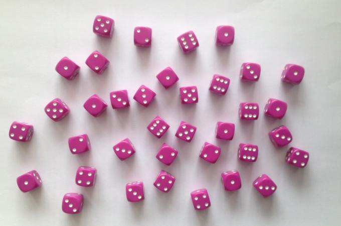
In this notebook, we just introduce a few classical image processing operations while playing with dice. The goal of the example is to count the total score one the dice, the answer being \(113\).
%matplotlib widget
from PIL import Image
import numpy as np
import matplotlib.pyplot as plt
from matplotlib import cm
from scipy import ndimage
import pandas as pd
import os
You can download the image used in this example here (just right-click and download):
The following code will work if the image is located in the same directory as the notebook itself.
First, let’s check if the file “dice.jpg” is in the current directory.
Ok, the file is in ['HSLA_340.jpg', 'exercises.md', 'image_processing_tutorial.ipynb', 'image_processing_practical_work_bonus.ipynb', 'image_processing_practical_work.ipynb', 'dice.jpg', 'coins.jpg']
Now let’s read it using Python Image Library (aka PIL):
im = Image.open(path)
Nc, Nl = im.size
im = im.resize((Nc // 2, Nl // 2))
fig, ax = plt.subplots()
ax.axis("off")
plt.imshow(im)
plt.show()
Conversion to grayscale#
R, G, B = im.split()
R = np.array(R)
G = np.array(G)
B = np.array(B)
R
array([[222, 222, 222, ..., 198, 196, 196],
       [223, 223, 223, ..., 198, 196, 196],
       [224, 224, 224, ..., 198, 196, 196],
       ...,
       [231, 231, 231, ..., 193, 193, 193],
       [231, 231, 231, ..., 193, 193, 193],
       [232, 230, 230, ..., 191, 191, 193]], shape=(225, 340), dtype=uint8)
title_list = [
    "Red channel",
    "Green channel",
    "Blue channel",
]
fig, axs = plt.subplots(nrows=1, ncols=3)
fig.tight_layout(pad=3.0)
for i in range(3):
    axs[i].imshow(np.array(im)[:, :, i], cmap="gray")
    axs[i].title.set_text(title_list[i])
The green channel has a great contrats so we chose to work only on this channel now.
Histogram#
The histogram shows the repartition of the pixels on the color scale.
plt.figure()
plt.hist(G.flatten(), bins=np.arange(255))
plt.title("Green channel histogram")
plt.xlabel("Pixel value")
plt.ylabel("Count")
plt.show()
Thresholding#
Using the histogram, one can see that there are 3 peaks. The left peak is the darkest one and corresponds to the colors of the dice bodies. We can cut around \(120\) to isolate the dice bodies from the pips on the dice.
Further reading: Thresholding (Scikit)
import ipywidgets as widgets
import matplotlib.pyplot as plt
import numpy as np

# set up plot
fig, ax = plt.subplots(figsize=(6, 4))


@widgets.interact(low_tresh=(0, 255, 1))
def update(low_tresh=120):
    """Remove old lines from plot and plot new one"""
    plt.cla
    Gb = np.zeros_like(G)
    Gb = np.where(G > low_tresh, 1, Gb)
    ax.imshow(Gb, cmap="binary")
Erosion / Dilation#
# CODE HERE
Labeling#
# CODE HERE