from scipy.integrate import odeint
Simple pendulum#
Author: Ludovic Charleux (ludovic.charleux@univ-smb.fr)
Background#
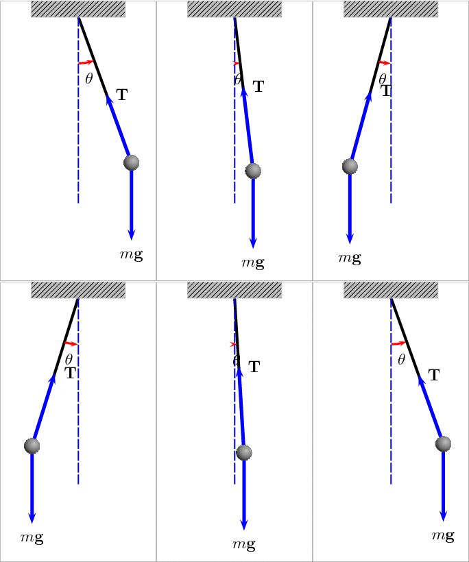
This tutorial aims to model and simulate the oscillations of a simple pendulum. A representation is given below (source: Wikipedia).

The pendulum consists of a point mass \(m\) located at the point \(M\) attached to a rigid arm considered without mass. The length of the arm is noted \(L\). This arm is articulated with respect to a frame considered as an inertial reference frame. The angle between the arm and the vertical direction is noted \(\theta\). A simple modeling using dynamics leads to :
Where:
\(\vec A(M/0)\) is the acceleration of the mass,
\(\vec P\) if the weight of the mass,
\(\vec T\) if the reaction force of the arm.
A projection of this equation along the direction perpendicular to the arm gives a more simple equation:
This equation is a non linear ODE of the second order whose exact solution is not known. It is however possible to assume that \(\theta\) is small enough to write that \(\sin \theta \approx \theta\). In this case, the equation comes down to the one of a free and undamped harmonic oscillator treated in the theoretical part. The object of this tutorial is to solve this problem by a numerical approach in a general way without simplifying assumptions.
L = 1.0  # m
g = 9.81  # m/s**2
Part 1: ODE reformulation#
This problem can be reformulated to match the standard formulation \(\dot X = f(X, t)\):
Write the function \(f\) in Python:
def f(X, t):
    """
    The simple pendulum's ODE
    """
    # CODE HERE !
    return
Part 2: solver validation at small angles#
In this first part, we want to validate the operation of the numerical solvers by comparing their results to a known exact solution. To do so, we will focus on the case of the simple pendulum oscillating at small angles. In this case, the sine can be approximated by \(\sin \theta \approx \theta\) and the equation of the pendulum can be reduced to that of a harmonic oscillator. The exact solution is then:
With:
\(X_0 = [\theta_0, 0]^T\)
\(\omega_0 = \sqrt{g/L}\)
Solve the problem with Euler, RK4 and ODEint integrators and compare the results with the closed form solution. First assume that the pendulum is released with no speed (\(\dot \theta = 0 ^o/s\)) at \(\theta = 1 ^o\). The time discretization will be as follows:
duration: from \(t_a = 0\) s to \(t_b = 10\) s.
time step: \(dt = 1. \times 10^{-2}\) s.
def Euler(func, X0, t):
    """
    Euler integrator.
    """
    dt = t[1] - t[0]
    nt = len(t)
    X = np.zeros([nt, len(X0)])
    X[0] = X0
    for i in range(nt - 1):
        X[i + 1] = X[i] + func(X[i], t[i]) * dt
    return X


def RK4(func, X0, t):
    """
    Runge and Kutta 4 integrator.
    """
    dt = t[1] - t[0]
    nt = len(t)
    X = np.zeros([nt, len(X0)])
    X[0] = X0
    for i in range(nt - 1):
        k1 = func(X[i], t[i])
        k2 = func(X[i] + dt / 2.0 * k1, t[i] + dt / 2.0)
        k3 = func(X[i] + dt / 2.0 * k2, t[i] + dt / 2.0)
        k4 = func(X[i] + dt * k3, t[i] + dt)
        X[i + 1] = X[i] + dt / 6.0 * (k1 + 2.0 * k2 + 2.0 * k3 + k4)
    return X


# ODEint is preloaded.
# Define the time vector t and the initial conditions X0
ta = 0.0
tb = 10.0
# CODE HERE
t = []  # REPLACE
theta = []  # REPLACE WITH YOUR SOLUTION

plt.figure()
plt.plot(t, np.degrees(theta))
plt.xlabel("Time, $t$")
plt.ylabel(r"Angular position, $\theta$ [$^o$]")
plt.grid()
Part 3: Anharmonic oscillations at larger energies#
In what follows, we work only with one of the solvers that has been sufficiently accurate in the previous section. We are interested in the operation of the pendulum at higher energy. First, increase the initial angle \(\theta_0\) to \(179^o\) and add an initial velocity. What do you observe about the shape of the curves (time, position) ?
# CODE HERE
theta = []  # REPLACE WITH YOUR SOLUTION

plt.figure("High energy")
plt.plot(t, np.degrees(theta))
plt.xlabel("Time, $t$")
plt.ylabel(r"Angular position, $\theta$ [$^o$]")
plt.grid()
Part 4 : Phase space#
For several initial conditions treated previously, draw the trajectory (integral curve) in the \((\theta, \dot \theta)\) phase plane. What remarkable points do you observe ?
theta = []  # REPLACE
dottheta = []  # REPLACE

plt.figure("Phase space")
plt.plot(np.degrees(theta), np.degrees(dottheta))
plt.xlabel(r"Angular position, $\theta$ [$^o$]")
plt.xlabel(r"Angular speed, $\dot\theta$ [$^o$]")
plt.grid()
Part 5: Conclusions#
Conclude on your observations on the following points: quality of the numerical solutions, shape of the integral curves, interest of the various representations used.
# ...


