Scientific Python

# UNCOMMENT FOR INTERACTIVE PLOTS
# %matplotlib notebook
import numpy as np
import pandas as pd
import matplotlib.pyplot as plt

def func(t, damp=1.0, freq=1.0, phase=0.0):
    """
    The solution of a second order linear ordinary differential equation:

    func(t) = exp(-t * damp) * cos(2 * pi * f * t + phase)

    Inputs:
    * damp: dampening coefficient.
    * freq: frequency
    * phase: the phase of the signal

    Ouput: data as a DataFrame for easier post processing.
    """
    return pd.DataFrame(
        {"a": np.exp(-t * damp) * np.cos(2.0 * np.pi * freq * t + phase), "t": t}
    )


t = np.linspace(0.0, 5.0, 1001)
data = func(t, damp=0.1, freq=1.0)
data.head()

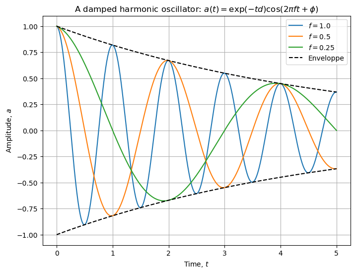
plt.figure(figsize=(8, 6))
for f in [1.0, 0.5, 0.25]:
    data = func(t, damp=0.2, freq=f)
    plt.plot(data.t, data.a, label="$f={0}$".format(f))
data = func(t, damp=0.2, freq=0)
plt.plot(data.t, data.a, "k--", label="Enveloppe")
plt.plot(data.t, -data.a, "k--")
plt.grid()
plt.legend(loc="best")
plt.xlabel("Time, $t$")
plt.ylabel("Amplitude, $a$")
plt.title(r"A damped harmonic oscillator: $a(t) = \exp(-t d) \cos (2 \pi f t + \phi)$")
plt.show()