Rosenbrock function and Curve fiting - POSITRON: PythOn for Science In The Reblochon cOuNtry

The Rosenbrock function¶

The Rosenbrock function is a classical benchmark for optimization algorithms. It is defined by the following equation:

f(x, y) = (1-x)^2 + 100 (y-x^2)^2

(1)

%matplotlib inline
import numpy as np
import matplotlib.pyplot as plt


def Rosen(X):
    """
    Rosenbrock function
    """
    x, y = X
    return (1 - x) ** 2 + 100.0 * (y - x**2) ** 2


x = np.linspace(-2.0, 2.0, 100)
y = np.linspace(-1.0, 3.0, 100)
X, Y = np.meshgrid(x, y)
Z = Rosen((X, Y))

fig = plt.figure(0)
plt.clf()
plt.contourf(X, Y, Z, 20)
plt.colorbar()
plt.contour(X, Y, Z, 20, colors="black")
plt.grid()
plt.xlabel("x")
plt.ylabel("y")
plt.show()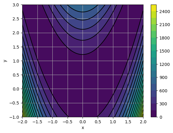

Questions¶

Find the minimum of the function using brute force. Comment the accuracy and number of function evaluations.
Same question with the simplex (Nelder-Mead) algorithm.

Curve fitting¶

Questions¶

Chose a mathematical function $y = f(x, a, b)$ and code it.
Chose target values of $a$ and $b$ that you will try to find back using optimization.
Evaluate it on a grid of $x$ values.
Add some noise to the result.
Find back $a$ and $b$ using curve_fit